In this article, I will use the Mercari Price Suggestion Data from Kaggle to predict store prices using Automated Differentiation Variational Inference, implemented in PyMC3. This price modeling was done by Susan Li in this article where she uses PyStan. Some of my work has been inspired by her code.

I’ll explain more about the dataset, the transformations that I perform, the models I chose and the accuracy that I have obtained from it. Note that the aim of this article is to explore different techniques to better model the prices and think about some of the ways to better structure the data. I won’t be implementing every single one of those techniques but I’ll be talking about them throughout the article.

The use-case for modeling prices

Every day, hundreds of new listings are released on e-commerce websites. The price of the listing makes a lot of difference because e-commerce websites have intensive competition, and it is very easy to lose a customer if the price of a listing is not within the general range of the affordability of an average customer. There are multiple factors that affect the viability of a product’s price. This includes the type of product, its condition, its brand and availability of services such as Free Shipping. In this assignment, we shall model the prices of these listings as a function of these factors.

Predicting the price of a listing can be very helpful for an e-commerce company because of the following reasons:

• A customer’s price decisions affect the online traffic that Mercari obtains, which is correlated to their reputation and profits from advertisements etc. Thus, the listing prices must be optimal and not randomly generated by a customer
• An informed price prediction helps the seller get significant customer attention which increases the chances of selling the product quickly without waiting for longer periods of time.
• A price-prediction tool also improves the product experience of a seller and a customer since the prices are reasonable and the seller does not have to spend a lot of energy in calculating the price and reducing it overtime to attract customers.
• Thus, price-prediction tools will have a significant impact on the experience of sellers and customers while boosting the profitability and reputation of Mercari.

The Data

The Data has been obtained from Mercari’s Kaggle Challenge to build a suggestion model that predicts the price of listings based on the information that a customer provides. The original dataset contains about 1.4 million data points. (Mercari, 2018)

For each data point, we have been provided with the following metrics:

• Condition ID: Specifies the condition of the product (Varies from 1 to 5).
• Name: The name of the listing
• Category Name: The general category of the product. There are about 1500 distinct categories.
• Brand Name: The name of the brand, or Nan if no brand.
• Price: The price listed by the customer.
• Shipping: If shipping is available
• Item Description: A description of the listing

Data Cleaning, Consolidation and Transformation

In order to analyze the data better, we perform a few operations to consolidate the text data:

• There are about 1500 different categories in the data. It is not realistic to model all these categories. Hence, I did not use sklearn’s Label Encoder which is the choice of many online model suggestions. Instead, I manually explored the data and made 8 major categories: Men, Women, Electronics, Sports, Beauty, Kids, Home and Other. Using keywords in the actual category, I classified each category as one of the eight major category codes.

# Loading and processing the data here
df = pd.read_csv(‘train.tsv’, sep=’\t’)
df = df[pd.notnull(df[‘category_name’])]
category_codes = []
# Analysing the words in each category and classifying them as either of the 8 numerical categories
for i in df.index:
    category = df['category_name'][i]
    
    if 'Men' in category:
        category_codes.append(0)
    elif 'Women' in category:
        category_codes.append(1)
    elif 'Electronics' in category:
        category_codes.append(2)
    elif 'Sports' in category:
        category_codes.append(3)
    elif 'Beauty' in category:
        category_codes.append(4)
    elif 'Kids' in category:
        category_codes.append(5)
    elif 'Home' in category:
        category_codes.append(6)
    else:
        category_codes.append(7)
df['category_code'] = category_codes

Note that the above approach is not the most optimal but it is a simple and efficient approach to sentiment analysis. One can go a lot deeper into the sentiment analysis of the category_name and the item_description of each product which would also reinforce the quality of the processed data. For example, one can analyze the presence of words such as ‘great condition’ or ‘works fine’ and give them a score/rating. The presence of different kinds of words would inform the total score of each product which can become a feature of our data.

• The condition id and shipping code were not changed since they are categorical variables that are ready for analysis.
• I won’t be using the item name for this analysis but it can also be processed using sentiment analysis to extract relevant information like size or features of the product that reinforce its price.
• For the brand, one can build a simple classifier that classifies bigger brands as ‘2’, smaller brands as ‘1’ and no brand as ‘0’. I won’t be implementing this strategy for the sake of simplicity in the model but I encourage you to try it.
• We convert the price onto a log-scale. This allows for a more smooth distribution over the prices which allows for easy modeling. This is also important because prices have something called a multiplicative factor. You can read more about it here. But essentially, prices change by multiplying them with a factor. For example, a price would get multiplied by a factor of 1.1 if shipping is available. Modeling these multiplicative factors is harder in Bayesian Statistics because they are much more likely to diverge during sampling. Hence, the log-scale converts the multiplicative factors into additive factors that we can model using linear regression. It also makes the price a continuous variable on the real number line.

Understanding the data better

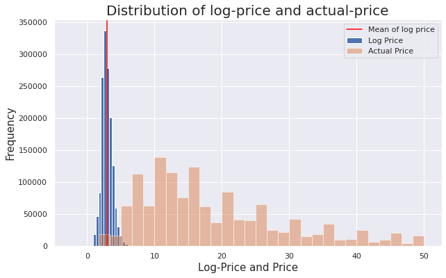
Let’s took a look at the price and the log-price distributions to see the transformation visually:

In the graph above, we can see that the distribution of log-price resembles a Normal distribution which is easier to model.

The graph above is quite interesting. The mean of prices for products with free shipping is actually smaller than the mean of prices for products with no free shipping, but we could expect the opposite because shipping should add to the cost of prices. There are two problems with that:

1. The distributions aren’t exactly Normal and hence, performing a t-test or comparing the means is not the best way to compare these distributions.
2. The comparative analysis here can be confounded as well. It may be the case that our data of products with no shipping contains cheaper products in general or contains a specific category of products that dominate the distribution. For example, most products with free shipping are usually cheaper (can be easily shipped as well) whereas heavier, bigger and costlier products don’t usually have free shipping. Thus, A $10 product with $2 shipping cost would be advertised as $12 but the costlier products are the ones with no shipping and their price (although not including the shipping cost) would be much higher than the cost of cheaper products that include shipping.

The above is a classic example of structural bias in the data that stems from the choices that we make as humans. As a data scientist, it is important to understand and account for these biases that stem from non-statistical choices. There’s no easy way to fix this bias. One way is to perform individual matching. Basically, we would run through the dataset and cherry-pick records that look exactly the same, or they’re very similar. The only main difference between them would be the availability of free shipping. Thus, we’ll construct a new dataset that contains two subsets, both with very similar distributions of products but one has no shipping while one has more shipping.

You can find the code for this visualization in the notebook at the end of the article. You are welcome to draw your own visualizations and reflect on biases that may be present in the dataset.

The Model

Let’s think about a simple linear regression first. (While linear regressions look very simple, they are powerful and scalable. Hence, data scientists prefer to process their data in a way that it can modelled using linear regression.)

Here, c is the constant in the model while a and b are the coefficients of shipping and condition. In an effort to make it realistic, I will be using pooling of the variables. This means that I will be creating a different value of a,b and c for each category of product. Hence, ‘Electronics’ will have its own set of parameters and ‘Home Decor’ will have its own set of parameters. This would be called partial-pooling if I didn’t do pooling for one or more of the parameters. Let’s update the equation:

Here, the [8] denotes that the parameters reflect 8 different parameters, one for each assigned category.

The meaning of a,b, and c:

We’ve built a model with a, b and c. But what do they mean? In terms of linear regression, c is the intercept while and b are the coefficients of condition and shipping. In terms of prices, ‘c’ is like the base price for each category. Each product in this category has a baseline or base price. This baseline is influenced by the condition of the product. The scale of this influence is controlled by ‘b’. The log price is further influenced by shipping. The scale of this influence is controlled by ‘a’

The Modeling infrastructure

Now that we have defined the basic structure of the model, we need to build the underlying prior distributions which are placed on these parameters. I will be using a hierarchical model here because hierarchy provides the flexibility of values and allows the different values of the same parameter to have their distribution rather than rely on the same one.

For example, each ‘a’ will be sampled from a Normal distribution of a mean and standard deviation, which are further sampled from their own priors. Thus, each ‘a’ will have its own Normal distribution which is important to satisfy the assumptions of pooling. Otherwise, they may get correlated which is a threat to the validity of the model.

Here, the hyperpriors of ‘a’ are mu and sigma. The mu is sampled from a Normal distribution whereas the standard deviation is sampled from a Uniform distribution between 0 and 10. Note that standard deviation must be positive and hence, we can’t use a Normal prior since the support of Normal distributions is the entire real number line. These priors have been chosen as uninformed priors because we do not know much about these coefficients or their effect. We will let the model find and converge over the best possible values.

We replicate the same model for ‘b’ and ‘c’ as well. We place a normal distribution on both of them which is further parameterized by their hyperparameters ‘ mu’ and ‘sigma’. Finally, the likelihood is modeled as another Normal distribution placed on the final linear equation with noise ‘sigma’.

Performing Inference

Now that we have established our model, we would like to perform inference in order to obtain the posterior distribution of a,b, and c which informs our ability to understand the model. We could allow MCMC to generate samples from it or we could perform Variational Inference where we place these distributions on our parameters and optimize for the values of their hyperparameters. Let’s reflect back on our goal from this analysis: Making a scalable inference on the prices of products.

Reflection on MCMC and its disadvantages:

A similar analysis was performed by Susan Li in this article where she uses PyStan. PyStan is a great tool that performs automated Hamiltonian Monte Carlo Sampling using a NUTS Sampler. But HMC is a very slow algorithm. In this dataset, we have about 1.4 million data points. This puts the average running time of the algorithm at about 2–3 hours. While there are different ways to optimize the efficiency of PyStan, it is not a scalable algorithm. You can learn more about Linear Regression in PyStan here.

Another important limitation of PyStan is the lack of scalable adaptability. We want our algorithms to update their parameters in real-time as new data is generated and processed so that the model becomes more intelligent every day. We also want this process to happen quickly and efficiently. Hence, PyStan may not be the best choice for an online marketplace model. You can read more about PyStan here.

Automated Differential Variational Inference

If you don’t know much about MCMC or Variational Inference (VI), you should read this article. To summarise, VI places a distribution on the given parameters and then optimizes these distributions.

VI uses something called KL-Divergence, which is a cost function and helps us understand the distance between what our result should look like, and where we want to be. But VI is not fully automated and requires fine-tuning. Thus, we’ll be using a version of VI called Automated Differentiation Variational Inference (ADVI) that optimizes a different parameter (similar to KL-Divergence but much easier to optimize). The algorithm uses different libraries to differentiate the ELBO (our metric here) and find the maxima to update the parameters. It uses coordinate descent (optimization along the coordinate axes) to achieve the parameter update equations. I know that was a lot of information, but I recommend you to read this article to get familiar with it.

An important note here: When we perform inference in VI, we perform inference over the variational parameters (here, the hyperparameters) that define the distribution of each Model parameter (a,b and c). Hence, the model variables become a transition parameter whose distributions are informed by inference over variational parameters (all the mu’s and all the sigma’s)

Building the model in PyMC3

For this implementation, we won’t be building an ADVI algorithm from scratch. Instead, we’ll be using PyMC3’s inbuilt features to build our model and specify the hyperpriors, the priors, the model and the inference strategy.

To make the inference faster, we’ll be using Minibatches in PyMC3. A Minibatch reduces the size of the training dataset. In an original setting, the parameter updates would require the parameters to look at the entire training dataset. Unfortunately, we have 1.4 million data points to look at. For about 25000 iterations (our goal), that’s a lot of work to do. Hence, Minibatches allow us to sample from the training dataset. They create a mini-batch of the training dataset (of size ‘b’) and the training for each update happens on the Mini-batch. The batches get updated after every iteration.

Over a significant number of iterations, Minibatches become very efficient at optimizing the ELBO since the update equations get to look at almost every single data point but not all at the same time which makes the process a lot more scalable.

Here is the code that builds the model for us. (I was inspired by this Hierarchical Partial Pooling Example provided on PyMC3’s website and some of the code has been adopted from their notebook.)

import pandas as pd
import matplotlib.pyplot as plt
import seaborn as sns; sns.set()
import numpy as np
%matplotlib inline
%env THEANO_FLAGS=device=cpu, floatX=float32, warn_float64=ignore
import theano
import theano.tensor as tt
import pymc3 as pm
category_code_new = df.category_code.values
shipping = df.shipping.values
condition_id = df.item_condition_id.values
log_price = df.log_price.values
n_categories = len(df.category_code.unique())
# Minibatches below. The batch size is 500
log_price_t = pm.Minibatch(log_price, 500)
shipping_t = pm.Minibatch(shipping, 500)
condition_t = pm.Minibatch(condition_id, 500)
category_code_t = pm.Minibatch(category_code_new, 500)
# Setting the hyperpriors (mu,sigma) for a,b,c
with pm.Model() as hierarchical_model:
    mu_a = pm.Normal('mu_alpha', mu=0., sigma=10**2)
    sigma_a = pm.Uniform('sigma_alpha', lower=0, upper=10)
    mu_b = pm.Normal('mu_beta', mu=0., sigma=10**2)
    sigma_b = pm.Uniform('sigma_beta', lower=0, upper=10)
    mu_c = pm.Normal('mu_c', mu=0., sigma=10**2)
    sigma_c = pm.Uniform('sigma_c', lower=0, upper=10)
# Setting the priors here. Note the shape variable.
# The shape must be equal the number of categories. (8 here)
with hierarchical_model:
    a = pm.Normal('alpha',mu=mu_a,sigma=sigma_a, shape=n_categories)
    b = pm.Normal('beta',mu=mu_b, sigma=sigma_b, shape=n_categories)
    c = pm.Normal('c', mu=mu_c, sigma=sigma_c, shape=n_categories)
# Setting the likelihood here as another gaussian
with hierarchical_model:
    # Estimated log prices
    log_price_est = c[category_code_t] + b[category_code_t] *
                     condition_t + a[category_code_t] * shipping_t
    # Noise or standard deviation of the likelihood
    noise = pm.Uniform('eps', lower=0, upper=100)
    #Likelihood function. Note that we still need to provide the 
    # total size of the dataset for convergence check.
    lp_like = pm.Normal('lp_like', mu=log_price_est, sigma=eps,
             observed=log_price_t, total_size=len(df))

Optimization time!

Let’s define the optimization strategy as ADVI in PyMC3 and perform the inference.

from pm.callbacks import CheckParametersConvergence
# Defining inference method and parameter checks
with hierarchical_model:
    inference = pm.ADVI()
    approx = pm.fit(100000, method=inference, callbacks= 
                    [CheckParametersConvergence()])
plt.figure(figsize=(12,6))
plt.plot(-inference.hist, label='new ADVI', alpha=.8)
plt.plot(approx.hist, label='old ADVI', alpha=.8)
plt.legend(fontsize=15)
plt.ylabel('ELBO', fontsize=15)
plt.xlabel('iteration', fontsize=15);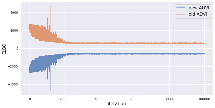

From the graph, we can say that the ELBO converged well and reached its minimum at around 25000 iterations. We observe minima at 490.22 whereas the maxima occurred at 4706.71. You might ask — What are the spikes in the ELBO around 10000 iterations. These are updates that have gone against our goal. It may have happened due to multiple reasons, most probably being a huge bias in the minibatch that caused the parameter update to skew from its trajectory. But its the beauty (and the math) of randomization that helps us reach the right result eventually.

Posterior Distributions of the Variational Parameters

Remember that we didn’t perform MCMC? Yes. So we won’t be getting samples but rather values of the variational parameters that are the hyperpriors of our model parameters, and then for the model parameters as well. The variable ‘approx’ that we got from fitting the model will provide us with the mean and the standard deviation for each parameter. We’ll obtain a dictionary of means and standard deviations that can be indexed with the parameter value:

means = approx.bij.rmap(approx.mean.eval())
sds = approx.bij.rmap(approx.std.eval())
a_mean = means['alpha']
a_std = sds['alpha'] # for each model and variational parameter

We aren’t very interested in the distributions of the variational parameters because their priors were not dynamic. We would take a quick glance at their means and standard deviations:

1. mu_a ~ N(-0.00022505, 0.7320357)
2. mu_b ~ N(6.097043e-05, 0.7320404)
3. mu_c ~ N(0.00212902, 0.7320338)

As expected, they are centered around 0 because the priors on these mu’s were also centered at 0. The standard deviations have readjusted themselves (from the original 10 to a lot smaller 0.732). All these mean distributions are very close to each other. Hence, the actual values of a,b, and c are being sampled from Gaussians that are very close to each other. The important thing to note is that, while the posterior on the means are similar, the actual posterior of the model parameters can be very different based on the inference performed.

Posterior Distributions of the Model Parameters

We use the following code to plot the PDF of the posterior distributions. (We can’t do histograms here because we don’t have a set of samples.)

from scipy import stats
# List of categories
category_names = ['Men','Women','Electronics','Sports','Beauty', 
                  'Kids', 'Home', 'Other']
# Model parameters names
model_param = ['alpha','beta','c']
fig, axs = plt.subplots(nrows=3, figsize=(12, 10))
# Plotting a set of PDFs for each Model parameter
for var, ax in zip(model_param, axs):
    mu_arr = means[var]
    sigma_arr = sds[var] 
    ax.set_title(var) # Title of the subplot
    for i, (mu, sigma) in enumerate(zip(mu_arr.flatten(),
                                 sigma_arr.flatten())):
        sd3 = (-4*sigma + mu, 4*sigma + mu)
        x = np.linspace(sd3[0], sd3[1], 300)
        y = stats.norm(mu, sigma).pdf(x) # PDF of the parameter
        ax.plot(x, y, label='Coefficient of {}'. format(
                                           category_names[i]))
    ax.legend()
fig.tight_layout()

Here are the posterior distributions for the pooled Model parameters:

Let’s analyze the model parameters:

1. For the base price (c), men’s clothing has the biggest baseline followed by women, home decor and Sports. Other products have the cheapest baseline. This is probably because of smaller miscellaneous products that do not have a lot of value as they are not part of any major category.
2. For the beta (b), the effects of the product condition are positive for some categories while they ate negative for others. More importantly, its a coefficient in a log-linear model. Hence, these coefficients represent the % change in the actual price. The highest negative effect of the bad condition is seen amongst Women’s clothing where a bad condition can lead to a 15% decline in price. The same applies to Men’s clothing and Home Decore. The decline is 5% for Sports and Kids’ clothing. There is an increase (about 12%) in the Electronics price with a bad condition which is counterintuitive but again, this would require matching for verification.
3. For the alpha (a), the effects of free shipping are largely negative (as we saw in the initial analysis before). Men’s clothing has the least negative effect (about -18%) whereas Electronics has the highest negative effect (about -50%). You should think more about the structural bias of the data and if the category reinforces the bias or not. Hint: Most electronics need more shipping/handling costs and hence, don’t offer free shipping.

From the above analysis, we can conclude that the most counterintuitive results were present in the category for Electronics and Other products whereas the rest of the products do not have as extreme results. It is worth performing matching on this dataset for better and more accurate modeling.

The uncertainties

From the posterior distributions, we can see that many of the distributions are very certain (such as the parameters of Women’s clothing). On the other hand, the parameters of Sports products are much more uncertain (Standard deviation of 0.025 which is approximately a 2.5% change in the actual price). Thus, as we build a predictive model from these results, we need to be careful about these uncertainties and incorporate them into our results.

A simple predictive model

We can technically build a deterministic predictive model from our results as a linear regression:

means = approx.bij.rmap(approx.mean.eval())
def predict(shipping, condition, category):
    c = means['c'][category]
    b = means['beta'][category]
    a = means['alpha'][category]
    return np.exp(c + b*condition + a*shipping)

But VI doesn’t provide us with prediction intervals while MCMC does. To obtain the prediction intervals, we simply need to build the confidence intervals for a,b, and c. Then, we use those intervals to evaluate the same predictions at the lower/upper bounds of a, b and c for the same inputs.

Comparison to results from HMC-NUTS Sampler

On the same model, we can also perform HMC-NUTS sampling to get posterior distributions. Here’s the code to accomplish that:

with hierarchical_model: 
    step = pm.NUTS(scaling=approx.cov.eval(), is_cov=True)
    hierarchical_trace = pm.sample(100000, step=step, 
                         start=approx.sample()[0], progressbar=True, 
                                    tune=1000, cores=4)
pm.summary(hierarchical_trace)

Note that PyMC3 has a few bugs with their NUTS Sampler (mainly with the summary function) and hence, I haven’t used it extensively but you can still get some good insights into the convergence of our results using MCMC.

Spoiler Alert: The chains will not converge. The reason probably lies in the use of MiniBatches which causes the chains to diverge because MCMC doesn’t exactly work to perform iterations of updating parameters. It works to create a number of samples that you want to generate. Hence, this set of samples can become very different if the samples are generated based on different Minibatches (which is the case). You would need a lot more iterations and chains to accomplish convergence in this case.

Future steps and Improvements

There are many ways to improve the current model. We discussed some of the ways to analyze text data better. Here are some things that Mercari could do better in terms of data collection:

1. Mercari could also do a better job of collecting more data that is accurate and easy to process. Instead of asking for a typed description, we can set up 5 questions that help the user classify the product better. This would also allow us to collect good data that can be easily analyzed. For example, we could ask questions like ‘How old is the product?’, ‘Does the product work?’, ‘Is it refurbished or Does it come with a warranty?’, ‘How much did you pay for it when you bought it?’. etc.

2. A customer’s preferences should also be taken into account for building a price predictor. Each customer has certain preferences in terms of waiting time, price expected, the price paid initially, emotional/social value (belonged to a celebrity), etc. Thus, the price should be adjusted based on the preferences and profile of the customer.

Testing Notebook

Feel free to clone the Python Notebook here and test different strategies.

Note: If you have any questions or if you’d like to connect, my LinkedIn profile is here.